이번 포스팅에서는 포자랩스에서 핵심적으로 쓰고 있는 모델인 transformer의 논문을 요약하면서 추가적인 기법들도 설명드리겠습니다.

Why?

Long-term dependency problem

sequence data를 처리하기 위해 이전까지 많이 쓰이던 model은 recurrent model이었습니다. recurrent model은 t번째에 대한 output을 만들기 위해, t번째 input과 t-1번째 hidden state를 이용했습니다. 이렇게 한다면 자연스럽게 문장의 순차적인 특성이 유지됩니다. 문장을 쓸 때 뒤의 단어부터 쓰지 않고 처음부터 차례차례 쓰는 것과 마찬가지인것입니다.
하지만 recurrent model의 경우 많은 개선점이 있었음에도 long-term dependency에 취약하다는 단점이 있었습니다. 예를 들어, “저는 언어학을 좋아하고, 인공지능중에서도 딥러닝을 배우고 있고 자연어 처리에 관심이 많습니다.”라는 문장을 만드는 게 model의 task라고 해봅시다. 이때 ‘자연어’라는 단어를 만드는데 ‘언어학’이라는 단어는 중요한 단서입니다.
그러나, 두 단어 사이의 거리가 가깝지 않으므로 model은 앞의 ‘언어학’이라는 단어를 이용해 자연어’라는 단어를 만들지 못하고, 언어학 보다 가까운 단어인 ‘딥러닝’을 보고 ‘이미지’를 만들 수도 있는 거죠. 이처럼, 어떤 정보와 다른 정보 사이의 거리가 멀 때 해당 정보를 이용하지 못하는 것이 long-term dependency problem입니다.
recurrent model은 순차적인 특성이 유지되는 뛰어난 장점이 있었음에도, long-term dependency problem이라는 단점을 가지고 있었습니다.
이와 달리 transformer는 recurrence를 사용하지 않고 대신 attention mechanism만을 사용해 input과 output의 dependency를 포착해냈습니다.

Parallelization

recurrent model은 학습 시, t번째 hidden state를 얻기 위해서 t-1번째 hidden state가 필요했습니다. 즉, 순서대로 계산될 필요가 있었습니다. 그래서 병렬 처리를 할 수 없었고 계산 속도가 느렸습니다.
하지만 transformer에서는 학습 시 encoder에서는 각각의 position에 대해, 즉 각각의 단어에 대해 attention을 해주기만 하고, decoder에서는 masking 기법을 이용해 병렬 처리가 가능하게 됩니다. (masking이 어떤 것인지는 이후에 설명해 드리겠습니다)

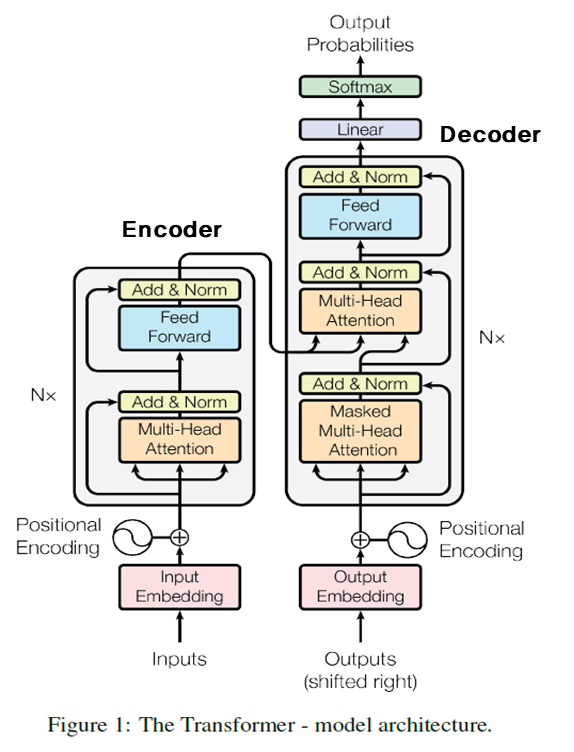
Model Architecture

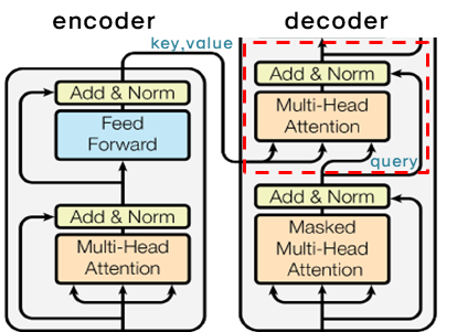
Encoder and Decoder structure

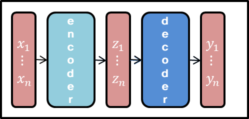
encoder는 input sequence $(x_{1}, . . ., x_{n})$ 에 대해 다른 representation인 $z = (z_{1}, . . ., z_{n})$ 으로 바꿔줍니다.
decoder는 z를 받아, output sequence $(y_{1}, . . ., y_{n})$ 를 하나씩 만들어냅니다.
각각의 step에서 다음 symbol을 만들 때 이전에 만들어진 output(symbol)을 이용합니다. 예를 들어, “저는 사람입니다.”라는 문장에서 ‘사람입니다’를 만들 때, ‘저는’이라는 symbol을 이용하는 거죠. 이런 특성을 auto-regressive 하다고 합니다.

Encoder and Decoder stacks

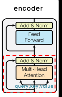
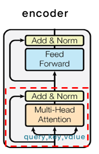
Encoder

N개의 동일한 layer로 구성돼 있습니다. input $x$가 첫 번째 layer에 들어가게 되고, $l a y e r (x)$ 가 다시 layer에 들어가는 식입니다.
그리고 각각의 layer는 두 개의 sub-layer, multi-head self-attention mechanism과 position-wise fully connected feed-forward network를 가지고 있습니다.
이때 두 개의 sub-layer에 residual connection을 이용합니다. residual connection은 input을 output으로 그대로 전달하는 것을 말합니다. 이때 sub-layer의 output dimension을 embedding dimension과 맞춰줍니다. $x + S u b l a y e r (x)$ 를 하기 위해서, 즉 residual connection을 하기 위해서는 두 값의 차원을 맞춰줄 필요가 있습니다. 그 후에 layer normalization을 적용합니다.

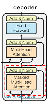
Decoder

역시 N개의 동일한 layer로 이루어져 있습니다.
encoder와 달리 encoder의 결과에 multi-head attention을 수행할 sub-layer를 추가합니다.
마찬가지로 sub-layer에 residual connection을 사용한 뒤, layer normalization을 해줍니다.
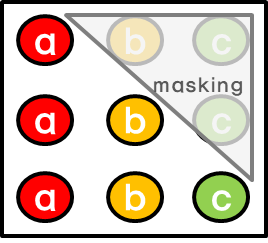
decoder에서는 encoder와 달리 순차적으로 결과를 만들어내야 하기 때문에, self-attention을 변형합니다. 바로 masking을 해주는 것이죠. masking을 통해, position $i$ 보다 이후에 있는 position에 attention을 주지 못하게 합니다. 즉, position $i$ 에 대한 예측은 미리 알고 있는 output들에만 의존을 하는 것입니다.

위의 예시를 보면, a를 예측할 때는 a이후에 있는 b,c에는 attention이 주어지지 않는 것입니다. 그리고 b를 예측할 때는 b이전에 있는 a만 attention이 주어질 수 있고 이후에 있는 c는 attention이 주어지지 않는 것이죠.

Embeddings and Softmax

embedding 값을 고정시키지 않고, 학습을 하면서 embedding값이 변경되는 learned embedding을 사용했습니다. 이때 input과 output은 같은 embedding layer를 사용합니다.
또한 decoder output을 다음 token의 확률로 바꾸기 위해 learned linear transformation과 softmax function을 사용했습니다. learned linear transformation을 사용했다는 것은 decoder output에 weight matrix $W$ 를 곱해주는데, 이때 $W$ 가 학습된다는 것입니다.

Attention

attention은 단어의 의미처럼 특정 정보에 좀 더 주의를 기울이는 것입니다.
예를 들어 model이 수행해야 하는 task가 번역이라고 해봅시다. source는 영어이고 target은 한국어입니다. “Hi, my name is poza.”라는 문장과 대응되는 “안녕, 내 이름은 포자야.”라는 문장이 있습니다. model이 이름은이라는 token을 decode할 때, source에서 가장 중요한 것은 name입니다.
그렇다면, source의 모든 token이 비슷한 중요도를 갖기 보다는 name이 더 큰 중요도를 가지면 되겠죠. 이때, 더 큰 중요도를 갖게 만드는 방법이 바로 attention입니다.

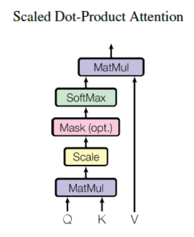
Scaled Dot-Product Attention

해당 논문의 attention을 Scaled Dot-Product Attention이라고 부릅니다. 수식을 살펴보면 이렇게 부르는 이유를 알 수 있습니다.

$A t t e n t i o n (Q, K, V) = s o f t m a x (\frac{Q K^{T}}{\sqrt{d_{k}}}) V$

먼저 input은 $d_{k}$ dimension의 query와 key들, $d_{v}$ dimension의 value들로 이루어져 있습니다.
이때 모든 query와 key에 대한 dot-product를 계산하고 각각을 $\sqrt{d_{k}}$ 로 나누어줍니다. dot-product를 하고 $\sqrt{d_{k}}$ 로 scaling을 해주기 때문에 Scaled Dot-Product Attention인 것입니다. 그리고 여기에 softmax를 적용해 value들에 대한 weights를 얻어냅니다.
key와 value는 attention이 이루어지는 위치에 상관없이 같은 값을 갖게 됩니다. 이때 query와 key에 대한 dot-product를 계산하면 각각의 query와 key 사이의 유사도를 구할 수 있게 됩니다. 흔히 들어본 cosine similarity는 dot-product에서 vector의 magnitude로 나눈 것입니다. $\sqrt{d_{k}}$ 로 scaling을 해주는 이유는 dot-products의 값이 커질수록 softmax 함수에서 기울기의 변화가 거의 없는 부분으로 가기 때문입니다.
softmax를 거친 값을 value에 곱해준다면, query와 유사한 value일수록, 즉 중요한 value일수록 더 높은 값을 가지게 됩니다. 중요한 정보에 더 관심을 둔다는 attention의 원리에 알맞은 것입니다.

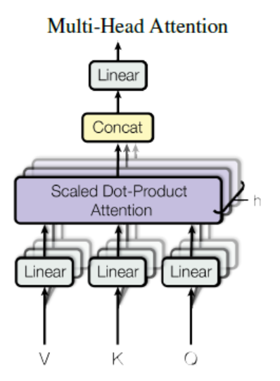
Multi-Head Attention

위의 그림을 수식으로 나타내면 다음과 같습니다.

$M u l t i H e a d (Q, K, V) = C o n c a t (h e a d_{1}, . . ., h e a d_{h}) W^{O}$

where $h e a d_{i} = A t t e n t i o n (Q W_{i}^{Q}, K W_{i}^{K}, V W_{i}^{V})$

$d_{m o d e l}$ dimension의 key, value, query들로 하나의 attention을 수행하는 대신 key, value, query들에 각각 다른 학습된 linear projection을 h번 수행하는 게 더 좋다고 합니다. 즉, 동일한 $Q, K, V$ 에 각각 다른 weight matrix $W$ 를 곱해주는 것이죠. 이때 parameter matrix는 $W_{i}^{Q} \in R^{d_{m o d e l} x d_{k}}, W_{i}^{K} \in R^{d_{m o d e l} x d_{k}}, W_{i}^{V} \in R^{d_{m o d e l} x d_{v}}, W_{i}^{O} \in R^{h d_{v} x d_{m o d e l}}$ 입니다.
순서대로 query, key, value, output에 대한 parameter matrix입니다. projection이라고 하는 이유는 각각의 값들이 parameter matrix와 곱해졌을 때 $d_{k}, d_{v}, d_{m o d e l}$ 차원으로 project되기 때문입니다. 논문에서는 $d_{k} = d_{v} = d_{m o d e l} / h$ 를 사용했는데 꼭 $d_{k}$ 와 $d_{v}$ 가 같을 필요는 없습니다.
이렇게 project된 key, value, query들은 병렬적으로 attention function을 거쳐 $d_{v}$ dimension output 값으로 나오게 됩니다.
그 다음 여러 개의 $h e a d$ 를 concatenate하고 다시 projection을 수행합니다. 그래서 최종적인 $d_{m o d e l}$ dimension output 값이 나오게 되는거죠.
각각의 과정에서 dimension을 표현하면 아래와 같습니다.

* $d_{Q}, d_{K}, d_{V}$ 는 각각 query, key, value 개수

Self-Attention

encoder self-attention layer

key, value, query들은 모두 encoder의 이전 layer의 output에서 옵니다. 따라서 이전 layer의 모든 position에 attention을 줄 수 있습니다. 만약 첫번째 layer라면 positional encoding이 더해진 input embedding이 됩니다.

decoder self-attention layer

encoder와 비슷하게 decoder에서도 self-attention을 줄 수 있습니다. 하지만 $i$ 번째 output을 다시 $i + 1$ 번째 input으로 사용하는 auto-regressive한 특성을 유지하기 위해 , masking out된 scaled dot-product attention을 적용했습니다.
masking out이 됐다는 것은 $i$ 번째 position에 대한 attention을 얻을 때, $i$ 번째 이후에 있는 모든 position은 $A t t e n t i o n (Q, K, V) = s o f t m a x (\frac{Q K^{T}}{\sqrt{d_{k}}}) V$ 에서 softmax의 input 값을 $- \infty$ 로 설정한 것입니다. 이렇게 한다면, $i$ 번째 이후에 있는 position에 attention을 주는 경우가 없겠죠.

Encoder-Decoder Attention Layer

query들은 이전 decoder layer에서 오고 key와 value들은 encoder의 output에서 오게 됩니다. 그래서 decoder의 모든 position에서 input sequence 즉, encoder output의 모든 position에 attention을 줄 수 있게 됩니다.
query가 decoder layer의 output인 이유는 query라는 것이 조건에 해당하기 때문입니다. 좀 더 풀어서 설명하면, ‘지금 decoder에서 이런 값이 나왔는데 무엇이 output이 돼야 할까?’가 query인 것이죠.
이때 query는 이미 이전 layer에서 masking out됐으므로, i번째 position까지만 attention을 얻게 됩니다.이 같은 과정은 sequence-to-sequence의 전형적인 encoder-decoder mechanisms를 따라한 것입니다.
*모든 position에서 attention을 줄 수 있다는 게 이해가 안되면 링크를 참고하시기 바랍니다.

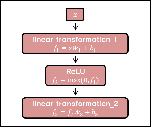
Position-wise Feed-Forward Networks

encoder와 decoder의 각각의 layer는 아래와 같은 fully connected feed-forward network를 포함하고 있습니다.

position 마다, 즉 개별 단어마다 적용되기 때문에 position-wise입니다. network는 두 번의 linear transformation과 activation function ReLU로 이루어져 있습니다.

$F F N (x) = m a x (0, x W_{1} + b_{1}) W_{2} + b_{2}$

$x$ 에 linear transformation을 적용한 뒤, $R e L U (m a x (0, z))$ 를 거쳐 다시 한번 linear transformation을 적용합니다.
이때 각각의 position마다 같은 parameter $W, b$ 를 사용하지만, layer가 달라지면 다른 parameter를 사용합니다.
kernel size가 1이고 channel이 layer인 convolution을 두 번 수행한 것으로도 위 과정을 이해할 수 있습니다.

Positional Encoding

transfomer는 recurrence도 아니고 convolution도 아니기 때문에, 단어의sequence를 이용하기 위해서는 단어의 position에 대한 정보를 추가해줄 필요가 있었습니다.
그래서 encoder와 decoder의 input embedding에 positional encoding을 더해줬습니다.
positional encoding은 $d_{m o d e l}$ (embedding 차원)과 같은 차원을 갖기 때문에 positional encoding vector와 embedding vector는 더해질 수 있습니다.
논문에서는 다른 *frequency를 가지는 sine과 cosine 함수를 이용했습니다.
*주어진 구간내에서 완료되는 cycle의 개수

$P E_{(p o s, 2 i)} = s i n (p o s / 10000^{2 i / d_{m o d e l}})$ $P E_{(p o s, 2 i + 1)} = c o s (p o s / 10000^{2 i / d_{m o d e l}})$

$p o s$ 는 position , $i$ 는 dimension 이고 주기가 $10000^{2 i / d_{m o d e l}} \cdot 2 π$ 인 삼각 함수입니다. 즉, $p o s$ 는 sequence에서 단어의 위치이고 해당 단어는 $i$ 에 0부터 $\frac{d_{m o d e l}}{2}$ 까지를 대입해 $d_{m o d e l}$ 차원의 positional encoding vector를 얻게 됩니다. $k = 2 i + 1$ 일 때는 cosine 함수를, $k = 2 i$ 일 때는 sine 함수를 이용합니다. 이렇게 positional encoding vector를 $p o s$ 마다 구한다면 비록 같은 column이라고 할지라도 $p o s$ 가 다르다면 다른 값을 가지게 됩니다. 즉, $p o s$ 마다 다른 $p o s$ 와 구분되는 positional encoding 값을 얻게 되는 것입니다.

$P E_{p o s} = [c o s (p o s / 1), s i n (p o s / 10000^{2 / d_{m o d e l}}), c o s (p o s / 10000)^{2 / d_{m o d e l}}, . . ., s i n (p o s / 10000)]$

이때 $P E_{p o s + k}$ 는 $P E_{p o s}$ 의 linear function으로 나타낼 수 있습니다. 표기를 간단히 하기 위해 $c = 10000^{\frac{2 i}{d_{m o d e l}}}$ 라고 해봅시다. $s i n (a + b) = s i n (a) c o s (b) + c o s (a) s i n (b)$ 이고 $c o s (a + b) = c o s (a) c o s (b) - s i n (a) s i n (b)$ 이므로 다음이 성립합니다.
$P E_{(p o s, 2 i)} = s i n (\frac{p o s}{c})$

$P E_{(p o s, 2 i + 1)} = c o s (\frac{p o s}{c})$ $P E_{(p o s + k, 2 i)} = s i n (\frac{p o s + k}{c}) = s i n (\frac{p o s}{c}) c o s (\frac{k}{c}) + c o s (\frac{p o s}{c}) s i n (\frac{k}{c}) = P E_{(p o s, 2 i)} c o s (\frac{k}{c}) + c o s (\frac{p o s}{c}) s i n (\frac{k}{c})$ $P E_{(p o s + k, 2 i + 1)} = c o s (\frac{p o s + k}{c}) = c o s (\frac{p o s}{c}) c o s (\frac{k}{c}) - s i n (\frac{p o s}{c}) s i n (\frac{k}{c}) = P E_{(p o s, 2 i + 1)} c o s (\frac{k}{c}) - s i n (\frac{p o s}{c}) s i n (\frac{k}{c})$

이런 성질 때문에 model이 relative position에 의해 attention하는 것을 더 쉽게 배울 수 있습니다.
논문에서는 학습된 positional embedding 대신 sinusoidal version을 선택했습니다. 만약 학습된 positional embedding을 사용할 경우 training보다 더 긴 sequence가 inference시에 입력으로 들어온다면 문제가 되지만 sinusoidal의 경우 constant하기 때문에 문제가 되지 않습니다. 그냥 좀 더 많은 값을 계산하기만 하면 되는거죠.

Training

training에 사용된 기법들을 알아보겠습니다.

Optimizer

많이 쓰이는 Adam optimizer를 사용했습니다.
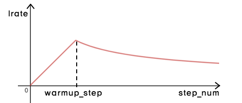
특이한 점은 learning rate를 training동안 고정시키지 않고 다음 식에 따라 변화시켰다는 것입니다.

$l r a t e = d_{m o d e l}^{- 0.5} \cdot m i n (s t e p_n u m^{- 0.5}, s t e p_n u m \cdot w a r m u p_s t e p s^{- 1.5})$

$w a r m u p_s t e p$ 까지는 linear하게 learning rate를 증가시키다가, $w a r m u p_s t e p$ 이후에는 $s t e p_n u m$ 의 inverse square root에 비례하도록 감소시킵니다.
이렇게 하는 이유는 처음에는 학습이 잘 되지 않은 상태이므로 learning rate를 빠르게 증가시켜 변화를 크게 주다가, 학습이 꽤 됐을 시점에 learning rate를 천천히 감소시켜 변화를 작게 주기 위해서입니다.

Regularization

Residual Connection

Identity Mappings in Deep Residual Networks라는 논문에서 제시된 방법이고, 아래의 수식이 residual connection을 나타낸 것입니다.

$y_{l} = h (x_{l}) + F (x_{l}, W_{l})$ $x_{l + 1} = f (y_{l})$

이때 $h (x_{l}) = x_{l}$ 입니다. 논문 제목에서 나온 것처럼 identity mapping을 해주는 것이죠.
특정한 위치에서의 $x_{L}$ 을 다음과 같이 $x_{l}$ 과 residual 함수의 합으로 표시할 수 있습니다.

$x_{2} = x_{1} + F (x_{1}, W_{1})$ $x_{3} = x_{2} + F (x_{2}, W_{2}) = x_{1} + F (x_{1}, W_{1}) + F (x_{2}, W_{2})$ $x_{L} = x_{l} + \sum_{i = 1}^{L - 1} F (x_{i}, W_{i})$

그리고 미분을 한다면 다음과 같이 됩니다.

$\frac{σ ϵ}{σ x_{l}} = \frac{σ ϵ}{σ x_{L}} \frac{σ x_{L}}{σ x_{l}} = \frac{σ ϵ}{σ x_{L}} (1 + \frac{σ}{σ x_{l}} \sum_{i = 1}^{L - 1} F (x_{i}, W_{i}))$

이때, $\frac{σ ϵ}{σ x_{L}}$ 은 상위 layer의 gradient 값이 변하지 않고 그대로 하위 layer에 전달되는 것을 보여줍니다. 즉, layer를 거칠수록 gradient가 사라지는 vanishing gradient 문제를 완화해주는 것입니다.
또한 forward path나 backward path를 간단하게 표현할 수 있게 됩니다.

Layer Normalization

Layer Normalization이라는 논문에서 제시된 방법입니다.

$μ^{l} = \frac{1}{H} \sum_{i = 1}^{H} a_{i}^{l}$ $σ^{l} = \sqrt{\frac{1}{H} \sum_{i = 1}^{H} (a_{i}^{l} - μ^{l})^{2}}$

같은 layer에 있는 모든 hidden unit은 동일한 $μ$ 와 $σ$ 를 공유합니다.
그리고 현재 input $x^{t}$ , 이전의 hidden state $h^{t - 1}$ , $a^{t} = W_{h h} h^{t - 1} + W_{x h} x^{t}$ , parameter $g, b$ 가 있을 때 다음과 같이 normalization을 해줍니다.

$h^{t} = f [\frac{g}{σ^{t}} ⊙ (a^{t} - μ^{t}) + b]$

이렇게 한다면, gradient가 exploding하거나 vanishing하는 문제를 완화시키고 gradient 값이 안정적인 값을 가짐로 더 빨리 학습을 시킬 수 있습니다.
(논문에서 recurrent를 기준으로 설명했으므로 이에 따랐습니다.)

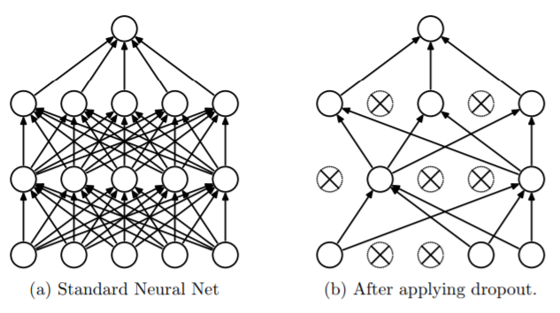
Dropout

Dropout: a simple way to prevent neural networks from overfitting라는 논문에서 제시된 방법입니다.

dropout이라는 용어는 neural network에서 unit들을 dropout하는 것을 가리킵니다. 즉, 해당 unit을 network에서 일시적으로 제거하는 것입니다. 그래서 다른 unit과의 모든 connection이 사라지게 됩니다. 어떤 unit을 dropout할지는 random하게 정합니다.
dropout은 training data에 overfitting되는 문제를 어느정도 막아줍니다. dropout된 unit들은 training되지 않는 것이니 training data에 값이 조정되지 않기 때문입니다.

Label Smoothing

Rethinking the inception architecture for computer vision라는 논문에서 제시된 방법입니다.
training동안 실제 정답인 label의 logit은 다른 logit보다 훨씬 큰 값을 갖게 됩니다. 이렇게 해서 model이 주어진 input $x$ 에 대한 label $y$ 를 맞추는 것이죠.
하지만 이렇게 된다면 문제가 발생합니다. overfitting될 수도 있고 가장 큰 logit을 가지는 것과 나머지 사이의 차이를 점점 크게 만들어버립니다. 결국 model이 다른 data에 적응하는 능력을 감소시킵니다.
model이 덜 confident하게 만들기 위해, label distribution $q (k ∣ x) = δ_{k, y}$ 를 (k가 y일 경우 1, 나머지는 0) 다음과 같이 대체할 수 있습니다.

$q^{'} (k | x) = (1 - ϵ) δ_{k, y} + ϵ u (k)$

각각 label에 대한 분포 $u (k)$ , smooting parameter $ϵ$ 입니다. 위와 같다면, k=y인 경우에도 model은 $p (y ∣ x) = 1$ 이 아니라 $p (y ∣ x) = (1 - ϵ)$ 이 되겠죠. 100%의 확신이 아닌 그보다 덜한 확신을 하게 되는 것입니다.

Conclusion

transformer는 recurrence를 이용하지 않고도 빠르고 정확하게 sequential data를 처리할 수 있는 model로 제시되었습니다.
여러가지 기법이 사용됐지만, 가장 핵심적인 것은 encoder와 decoder에서 attention을 통해 query와 가장 밀접한 연관성을 가지는 value를 강조할 수 있고 병렬화가 가능해진 것입니다.

Attention is all you need paper 뽀개기