조회수 3338
eventlet을 활용한 비동기 I/O 프로그래밍
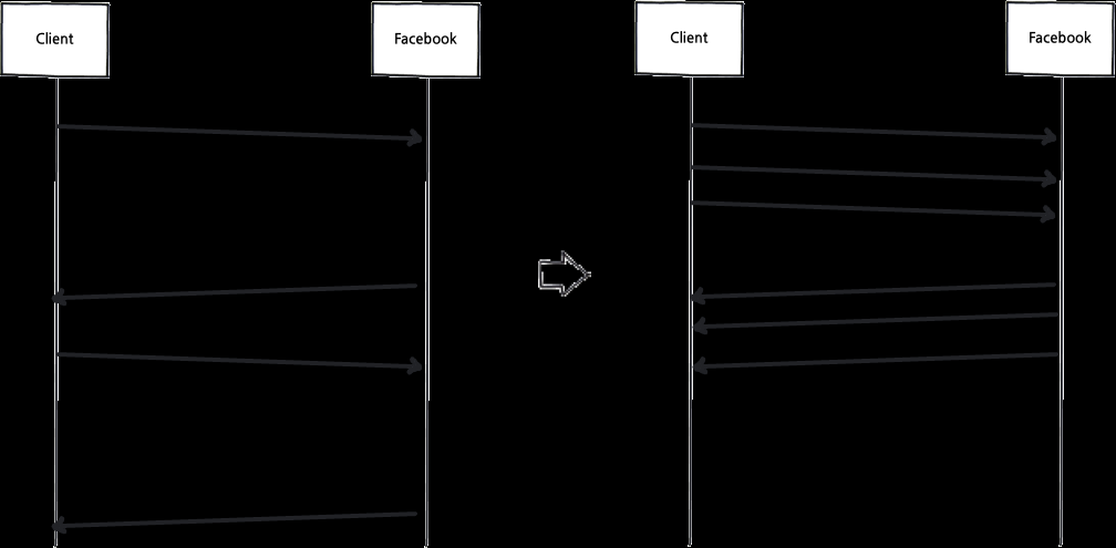
안녕하세요. 스포카 크리에이터팀 문성원입니다. 현대적인 프로그래밍 환경에서 네트워크는 더는 특정 직군의 개발자만 접하는 분야가 아닙니다. 그런 만큼 대량의 요청을 네트워크를 통해 송수신하는 프로그램이 생각보다 성능이 나오지 않는 경우를 경험하신 분들도 많으실 겁니다. 물론 스포카 개발팀도 예외는 아니었습니다. 그래서 오늘은 저희의 이러한 경험과 그 해결책-eventlet을 통한 비동기 I/O(Asynchronous I/O)-에 대해 소개합니다.Why우선 스포카 개발팀에서 겪었던 문제부터 시작하죠. 얼마 전 페이스북(facebook)의 FQL(Facebook Query Language)를 통해 정보를 수집해서 이를 활용하는 기능을 작성해야 했습니다. 기존의 함수들은 필요할 때마다 FQL을 요청하는 방식이었고 당연히 이건 너무 느렸죠. 그래서 생각한 것이 “하루의 일정 시간마다 대량의 FQL 요청을 보내서 필요한 정보를 미리 갱신시켜놓자.”였습니다. 여기까진 좋았죠. 이때 제가 작성한 코드의 얼개를 살펴보면 대강 이렇습니다.# 페이스북 계정들을 가져와서 반복하면서for account in FacebookAccount.query: account.update() #FQL을 보내자.view rawgistfile1.py hosted with ❤ by GitHub그런데 문제가 있었습니다. 기존의 FQL을 보내는 FacebookAccount.update()는 FQL요청이 완료될때까지 멈추고 기다립니다. 대부분의 FQL요청이 2, 3초 정도 걸린다고 했을 때 이러한 지연은 매우 치명적입니다. 대안이 필요했고 자연스레 떠오른 것이 서두에 소개한 비동기 I/O(Asynchronous I/O)였습니다.Asynchronous과거 일부 고급 서버 개발자만 알고 있는(혹은 알아야 하는) 기술로 치부되던 ‘비동기(Asynchronous)’란 개념은 2000년대 들어 등장한 Ajax(Asynchronous JavaScript and XML)의 성공 이후 많은 개발자에게 강한 인상을 줬습니다. 사용자는 HTTP 요청이 끝날 때까지 멈추어 있는 하얀 화면으로부터 해방되었고, 다양하고 많은 요청과 응답들이 자연스럽게 서버로 흘러들어 가서 나왔습니다. 개발자들의 이러한 경험과 통찰은 이후 node.js와 같은 플랫폼의 등장에도 많은 영향을 끼쳤습니다.다시 문제로 돌아가죠. 그렇다면 이러한 비동기에 관한 개념은 위의 상황을 어떻게 해결할 수 있을까요? 문제의 원인부터 다시 살펴봅시다. 2, 3초 정도씩 걸리는 FQL 요청이 문제일까요? 물론 요청이 매우 빨리 처리된다면 별도의 처리 없이도 저 코드는 문제없이 동작합니다. 하지만 현실적으로 이런 I/O의 속도를 빠르게 하는데에는 물리적으로 한계가 있습니다. 오히려 여기에서 주목해야 할 점은 ‘2, 3초’ 보다 ‘기다린다’라는 점입니다. FacebookAccount.update() 같은 경우, I/O가 처리되는 동안 CPU는 하던 일을 멈추고 문자 그대로 기다리게 됩니다. 만약 CPU가 멈추지 않고 다른 요청을 보낸다면 어떨까요? 이렇게 말이죠.비동기만으로는 부족하다?이러한 아이디어는 그동안 많은 개발자가 대량의 I/O를 다루는 올바른 방식으로 여겨왔습니다. 하지만 보통 이러한 비동기 I/O를 통한 구현은 동기식 I/O와는 좀 다른 형태를 띠게 됩니다. 이렇게 말이죠.# http://docs.python.org/library/asyncore.html#asyncore-example-basic-http-clientimport asyncore, socketclass HTTPClient(asyncore.dispatcher): def __init__(self, host, path): asyncore.dispatcher.__init__(self) self.create_socket(socket.AF_INET, socket.SOCK_STREAM) self.connect( (host, 80) ) self.buffer = 'GET %s HTTP/1.0\r\n\r\n' % path def handle_connect(self): pass def handle_close(self): self.close() def handle_read(self): print self.recv(8192) def writable(self): return (len(self.buffer) > 0) def handle_write(self): sent = self.send(self.buffer) self.buffer = self.buffer[sent:]client = HTTPClient('www.python.org', '/')asyncore.loop()view rawgistfile1.py hosted with ❤ by GitHub불행하게도, 이 경우 기존에 사용하던 urllib2대신 HTTP 요청을 처리하는 핸들러를 이처럼 재작성 해야합니다. 거기에 FacebookAccount.update()의 호출 방식마저 바뀔 수 있죠. 더군다나 콜백(Callback) 투성이의 코드는 유지보수가 쉬어 보이지도 않습니다. 여러모로 손이 많이 가는 상황이죠.결국, 기존 코드를 최대한 수정하지 않으면서도, 어느 정도 성능은 보장되는 그런 해결책이 필요했습니다. 그런 해결책이 있을까요? 다행히도 그렇습니다.What저희가 해결책으로 택한 eventlet은 Python(정확히는 CPython)에서 코루틴(Coroutine)을 지원하기 위해 만들어진 greenlet을 이용해 작성된 네트워크 관련 라이브러리입니다. 생소한 용어가 갑자기 튀어나와서 놀라셨을지도 모르니 우선 eventlet에 대해 설명하기 전에 앞에 나온 용어들을 찬찬히 한번 살펴보죠.코루틴과 greenlet먼저 코루틴(Coroutine)부터 살펴보죠. 전산학도라면 누구나 그 이름을 한번은 들어봤을 도널드 카누쓰(Donald Knuth)는 자신의 저서 The Art of Computer Programming에서 코루틴을 다음과 같이 설명합니다.Subroutines are special cases of more general program components, called “coroutines.” In contrast to the unsymmetric relationship between a main routine and a subroutine, there is complete symmetry between coroutines, which call on each other.코루틴은 우리가 잘 알고 있는 서브루틴(Subroutine)과 달리 진입점(Entry Point)이 여러 개일 수 있습니다. 쉽게 이야기하면 실행을 멈췄다가(Suspend) 재개(Resume)할 수 있다는 점인데요. 이 특성을 살리면 우리가 익히 아는 스레드(Thread)처럼 쓸 수 있게 됩니다. 다만 스레드와 달리 코루틴은 비선점적(Non-Preemptive)이기때문에 코드의 흐름을 전적으로 사용자가 제어할 수 있습니다.하지만 불행히도 모든 언어에서 이런 코루틴이 지원되진 않습니다. greenlet은 이런 코루틴을 CPython에서 지원하기 위해 작성된 라이브러리입니다.eventlet코루틴을 통해 스레드를 대체할 수 있다는 점에 주목한 사람들은 greenlet을 통해 유용한 네트워크 라이브러리를 만들어냈습니다. eventlet도 그 중 하나죠. 잠시 eventlet의 소갯글을 봅시다.Eventlet is a concurrent networking library for Python that allows you to change how you run your code, not how you write it.위에서 볼 수 있듯이 eventlet은 사용성에 중점을 두었습니다. 기존의 블로킹 I/O 스타일의 프로그래밍에 익숙한 개발자들도 쉽게 비동기 I/O의 장점을 얻을 수 있게끔 하는 게 목적이죠.특히 저희가 주목한 점은 eventlet의 멍키패치 기능입니다. 멍키패치는 본래 동적 언어에서 런타임에 코드를 고쳐서 별도의 파일 변경 없이 본래 소스의 기능을 변경하는 것을 말합니다. eventlet은 eventlet.monkey_patch 메서드를 통해 표준 라이브러리의 I/O 라이브러리를 논블러킹으로 동작하게끔 변경해서 코루틴에 적합하게 만듭니다.How앞서 소개한 eventlet.monkey_patch를 이용하면 실제로 고칠 부분은 정말로 적어집니다. 다음 코드가 eventlet을 이용해 변경한 전부입니다.import eventleteventlet.monkey_patch() #표준 라이브러리를 변환# 여러가지 import를 하고...pool = eventlet.GreenPool()# 페이스북 계정들을 가져와서 반복하면서for account in FacebookAccount.query: # 코루틴들에게 떠넘기자. pool.spawn_n(FacebookAccount.update, account) pool.waitall()view rawgistfile1.py hosted with ❤ by GitHub정말 적죠? 조금만 구체적으로 살펴보죠. 우선 eventlet.monkey_patch는 socket이나 select등의 Python 표준 라이브러리를 eventlet.green 패키지안에 정의된 코루틴 친화적인 모듈들로 바꿔치기 합니다.# from eventlet/pathcer.pydef monkey_patch(**on): """Globally patches certain system modules to be greenthread-friendly. The keyword arguments afford some control over which modules are patched. If no keyword arguments are supplied, all possible modules are patched. If keywords are set to True, only the specified modules are patched. E.g., ``monkey_patch(socket=True, select=True)`` patches only the select and socket modules. Most arguments patch the single module of the same name (os, time, select). The exceptions are socket, which also patches the ssl module if present; and thread, which patches thread, threading, and Queue. It's safe to call monkey_patch multiple times. """ accepted_args = set(('os', 'select', 'socket', 'thread', 'time', 'psycopg', 'MySQLdb')) default_on = on.pop("all",None) for k in on.iterkeys(): if k not in accepted_args: raise TypeError("monkey_patch() got an unexpected "\ "keyword argument %r" % k) if default_on is None: default_on = not (True in on.values()) for modname in accepted_args: if modname == 'MySQLdb': # MySQLdb is only on when explicitly patched for the moment on.setdefault(modname, False) on.setdefault(modname, default_on) modules_to_patch = [] patched_thread = False if on['os'] and not already_patched.get('os'): modules_to_patch += _green_os_modules() already_patched['os'] = True if on['select'] and not already_patched.get('select'): modules_to_patch += _green_select_modules() already_patched['select'] = True if on['socket'] and not already_patched.get('socket'): modules_to_patch += _green_socket_modules() already_patched['socket'] = True if on['thread'] and not already_patched.get('thread'): patched_thread = True modules_to_patch += _green_thread_modules() already_patched['thread'] = True if on['time'] and not already_patched.get('time'): modules_to_patch += _green_time_modules() already_patched['time'] = True if on.get('MySQLdb') and not already_patched.get('MySQLdb'): modules_to_patch += _green_MySQLdb() already_patched['MySQLdb'] = True if on['psycopg'] and not already_patched.get('psycopg'): try: from eventlet.support import psycopg2_patcher psycopg2_patcher.make_psycopg_green() already_patched['psycopg'] = True except ImportError: # note that if we get an importerror from trying to # monkeypatch psycopg, we will continually retry it # whenever monkey_patch is called; this should not be a # performance problem but it allows is_monkey_patched to # tell us whether or not we succeeded pass imp.acquire_lock() try: for name, mod in modules_to_patch: orig_mod = sys.modules.get(name) if orig_mod is None: orig_mod = __import__(name) for attr_name in mod.__patched__: patched_attr = getattr(mod, attr_name, None) if patched_attr is not None: setattr(orig_mod, attr_name, patched_attr) # hacks ahead; this is necessary to prevent a KeyError on program exit if patched_thread: _patch_main_thread(sys.modules['threading']) finally: imp.release_lock()view rawgistfile1.py hosted with ❤ by GitHub이렇게 바꿔치기된 eventlet.green안의 모듈들은 I/O에 의해 블럭되는 경우 다른 코루틴에 제어권을 넘기는 식으로 지연을 방지합니다.다른 대안들사실 이러한 목적으로 사용되는 라이브러리는 eventlet만 있는 것은 아닙니다. gevent는 eventlet에서 영향을 받았지만, libevent를 기반으로 하여 더욱 나은 성능과 성숙한 인터페이스를 갖추고 있습니다. 저희처럼 libevent의 설치에 제한이 있는 환경이 아니라면 이쪽을 살펴보셔도 좋습니다.만약 이벤트 주도적 프로그래밍(Event-Driven Programming)에 흥미가 있으신 분은 Twisted역시 좋은 대안이 될 수 있습니다.#스포카 #개발 #개발자 #인사이트 #꿀팁


.jpeg)