NRSC-5-C is the standard for digital terrestial radio in the United States. The physical layer and protocols are well documented on the NRSC’s website. The audio compression details are conspicuously absent considering that the goal of the standard is digital audio.
Overview
The development goal of NRSC-5-C was digital terrestial radio using the already allocated FM bandwidth. The result was an IBOC (in-band on-channel) system that supports both analog and digital signals within the existing FM allocations. This hybrid scheme is flexible and the station can choose to allocate more or less of the spectrum to analog or digital. Eventually, the entire spectrum allocation could be used for a pure digital signal.

The system is split into several layers. The physical layer (layer 1) is responsible for finding the signal, decoding, and error correction. The multiplexer (layer 2) allows multiple layer 3 applications to share the bandwidth, giving priority to the real-time audio data. And the application layer (layer 3) is where the decoding of the audio data actually happens.
Our implementation of a NRSC-5 receiver is available in a GitHub repository. The source code is released under the GPL v3, and uses code from turbofec and reed-solomon, as well as the ao, faad2, and liquid-dsp libraries.
Layer 1
The physical layer has similarities to other digital systems like DVB, LTE, and Wi-Fi. OFDM is used to multiplex 1093 subcarrier signals, which modulate the data using either DBPSK or QPSK. A cyclic prefix is inserted to aid synchronization, and the digital data is scrambled, encoded with a convolutional code, and interleaved to protect the data from errors. The total bandwidth reserved for the digital signal is determined by the operating mode, but generally the digial signal is split across two sidebands of 69 KHz each, resulting in a 96 kbps channel.

Parameters
| Parameter Name | Units | Exact Value |
|---|---|---|
| OFDM Subcarrier Spacing | Hz | |
| Cyclic Prefix Width | none | |
| OFDM Symbol Duration | seconds | |
| Sample Rate | samples / second | 744187.5 |
| OFDM Subcarriers | none | 2048 |
| Cyclic Prefix Width | samples | 112 |
| OFDM Symbol Duration | samples | 2160 |
Filtering
The first step is to receive the signal at the center frequency for the radio station, and filter out the analog audio. We chose to receive the signal at twice the sample rate, ~1.488 MHz, and use a decimating band-pass filter to eliminate the analog audio and act as an anti-aliasing filter. The filter does not need to be exact; the filter taps we used allow frequencies 122457 Hz - 372095 Hz to pass through. Eliminating the analog audio makes it easier for the timing synchronization and frequency error correction in the next steps.

Synchronization
Once we have a signal at the correct sample rate and approximately the correct frequency, we can use autocorrelation to find the start of the cyclic prefix. One of the prolems with OFDM is that even small timing offsets or frequency errors will result in the loss of orthogonality and corrupted data. Thankfully, we can fix both of these issues using the cyclic prefix that was inserted by the transmitter.

A cyclic prefix is a copy of the last few samples of the OFDM symbol inserted at the beginning of the OFDM symbol. This will make the OFDM symbol longer, which reduces bandwidth, but it also enables autocorrelation to find the beginning of the OFDM symbol and acts as a guard interval to prevent intersymbol interference. Autocorrelation (wikipedia) is a simple technique whereby the signal is correlated (wikipedia) with a delayed copy of itself and we look for a peak. In the case of a cyclic prefix, the delay is the length of the original OFDM symbol, 2048 samples.

The peak of the correlation finds the point where the same signal is present in both the delayed and non-delayed signals. Because the data is pseudorandom, the only time this should happen is when the delayed signal is at the cyclic prefix and the non-delayed signal is near the end of the OFDM signal. This tells us the timing offset, or which sample is the beginning of the OFDM symbol, and we can now strip off the cyclic prefix samples.
The result of the correlation also enables minor correction of the frequency of the signal. If there is “small” frequency offset, then it will introduce a phase shift between the cyclic prefix and the matching samples at the end of the symbol. This phase shift is the complex argument, or phase angle, of the correlation. Since there are 2048 samples between the cyclic prefix and the matching samples, and the sample rate is 744187.5, we can estimate the frequency offset as:
Lastly, the timing offset we found earlier can also help us correct for small differences in the sample rate. Because the oscillators in the transmitter and receiver are not perfectly in sync, the sample rates are slightly different. This manifests itself as a change in the timing offset over time. If the timing offset decreases, then the receiver sample rate is too low, and if the offset is increasing then the sample rate is too high. We use this observation and an arbitrary resampler to try to syncronize the sample rates and keep the timing offset constant over time.
OFDM Decoding
Once we have the corrected OFDM symbol without the cyclic prefix, we can use a FFT to recover the 2048 subcarrier signals. Not all of these subcarriers are used, in fact we ignore most of them. In this system, there are two types of subcarriers: reference subcarriers and data subcarriers. The reference subcarriers contain a repeating DBPSK modulated signal that can be used for channel estimation and block synchronization. The data subcarriers contain the encoded data which is modulated using QPSK.
The signal that we received and used to recover the subcarriers was not the originally transmitted signal due to noise and multipathing. The process of channel estimation is figuring out how the signal was corrupted so that we can remove the error from the subcarrier signals. Because the reference subcarriers are modulated using DPBSK and contain sync bits that are always the same, we can determine the change in amplitude and the change in phase for each reference subcarrier. Using this information we can estimate the error signal and recover the orignal reference signal.
The reference subcarriers are spread out so that there is always a partition of 18 data subcarriers with a reference subcarrier on each side. Since we can determine the changes to the amplitude and phase of the two reference subcarriers, we can estimate the error for each data subcarrier using linear interpolation and remove the error from the signals. Other interpolation methods are possible, but linear interpolation is one of the simplest and is effective. After the error correction, we can demodulate the QPSK signals to recover the data bits.
Reference Subcarriers
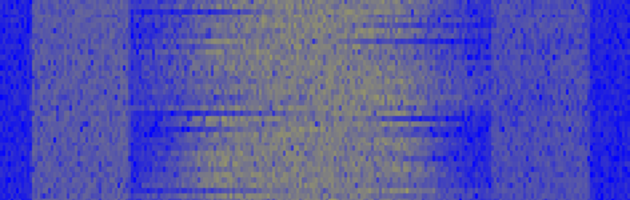
The reference subcarriers are modulated using differential binary phase shift keying (DBPSK). Using DBPSK makes the reference data more resilient to phase shifts because there are only two possible original symbols: -1+0i, 1+0i. The reference data also contains several sync bits that can be used by the receiver to find the beginning of the reference data, determine if the phase is shifted by 180 degrees, and correct for coarse frequency offset. The diagram below labels each bit in the reference data along with their static values to find the first block of the 0th reference subbcarrier.

Interleaving
There are several service modes which determine how many subcarriers are in-use and how the subcarriers are assigned to the logical channels (P1, P2, P3, P4, PIDS). The P1 logical channel contains the actual audio data and is the one we will focus on. There is an additional logical channel, PIDS, which contains the station information and is always present.
The logical channels are interleaved in order to diffuse any burst errors across the L1 frames. The deinterleaver receives 16 interleaver blocks, where each interleaver block is the data bits from the data subcarriers across 32 OFDM symbols. The MP1 hybrid service mode has 10 subcarrier partitions in the lower and upper sideband, which gives a total of 360 data subcarriers, or 720 bits using QPSK modulation. So the interleaver will receive bits, and using the PM interleaver matrix, we will get 1 P1 transfer frame (365440 bits) and 16 PIDS transfer frames (200 bits each).
The interleaver matrix definition is tedious but straightforward; refer to page 74 of the layer 1 reference documentation. One issue we encountered during implementation was a reversal of the row bits, so we needed to adjust the deinterleaver to compensate.
Viterbi Decoding
Once we have a complete P1 transfer frame, we need to decode it to get the original transfer frame. The P1 transfer frame is encoded with a 2/5 punctured convolutional code using a 1/3 tail-biting mother code. We can decode it by first depuncturing, then using a Viterbi decoder.
One of the benefits of a Viterbi decoder is that it can be a soft-decision decoder, so the previous QPSK demodulation step can output a probability instead of a fixed value. For instance, we can represent the output of the QPSK demodulation step as two signed 8-bit values in the range [-127, 127], where -127 represents a definite 0-bit, 127 represents a definite 1-bit, and 0 is unknown. We will refer to these 8-bit values as soft-bits.
To depuncture the input, we insert in an unknown soft-bit (for instance, 0) after every 5th soft-bit from the input. This has the effect of expanding the transfer frame from 365440 bits to 438528 bits. This maps to the 2/5 puncture matrix on page 45, and might be different for other channels (e.g. P3 and P4).
The frame can now be passed into a Viterbi decoder for the 1/3 mother code. A M/N code has M input bits for N output bits. Since we are decoding a block of 438528 bits, the original input size was 146176 bits. Also, a convolutional code has a constraint length (K=7) which determines how many input bits influence the next output bit. The complete parameters are in the table below, and generally match the parameters used by LTE.
| M | N | K | Generator Polynomials | Length | Termination |
|---|---|---|---|---|---|
| 1 | 3 | 7 | [0133, 0171, 0165] | 146176 | Tail-biting |
A complete description and understanding of Viterbi decoding is unnecessary. We used the TurboFEC Library from Ettus Research since the parameters are similar to those used by LTE. The basic idea is that it performs a maximum likelihood decoding to guess the correct input bits given the output bits and their likelihood. As shown in the diagram below, each output bit depends on 7 input bits. Input represents the current input bit, and input represents the previous -th input bit. These relationships enable the decoder to guess the original input bits.

Scrambling
The system uses a fibonacci linear feedback shift register (LFSR) to generate pseudorandom bits which are used to scramble the data before encoding. The LFSR uses a primitive polynomial of with an initial state of all ones. A basic implementation of the LFSR looks like:
1 2 3 4 5 6
unsigned int state = 0x3ff; while (true) { int output = ((state >> 9) ^ state) & 1; state = ((output << 11) | state) >> 1; // use output }
Descrambling the data is as simple as perfoming 146176 iterations of the loop, and XOR the output of the LFSR with the data. The result is the frame data from Layer 2.
Layer 2
The multiplexer allocates the audio data and other payloads to the various Layer 1 logical channels (e.g. P1, P3, P4, PIDS). The idea is to reserve as much bandwidth as necessary for the audio data (MPS PDUs and SPS PDUs), and include other data opportunistically if there is spare bandwidth. The MPS PDU always comes first in the Layer 2 output (L2 PDU) followed by the SPS PDUs and then any opportunistic data. The exception is the PIDS logical channel which will only carry station information PDUs.
One of the features of the switch to digital audio is the capability to have multiple programs using the same bandwidth. These programs are referred to by their station and program number, for instance KUT HD3 or 90.5-3. The program number used internally is base-0 whereas the public program number is base-1, so the main program, HD1, is actually program number 0. The MPS PDU always contains the main program (0) and the SPS PDUs contain the secondary programs (1 - 7).
The L2 PDU contains a 24-bit value (PCI) whose bits are spread out across the L2 PDU. The PCI indicates whether there is audio data, fixed data, and/or opportunistic data. We are only interested in decoding the audio data from logical channel P1, so we know there will always be audio data and we can ignore the PCI value, but we still need to remove it to extract the MPS/SPS PDUs. To remove the PCI value from a P1 L2 PDU, remove the bits at offsets [116176, 117424, …, 144880]. Page 13 of the layer 2 reference documentation has the generic algorithm to handle other L2 PDUs and the valid PCI values are below.
| Sequence | Hex Value | Audio Data | Fixed Data | Opportunistic Data |
|---|---|---|---|---|
| 0x38D8D3 | Yes | No | No | |
| 0xCE3634 | Yes | No | Yes | |
| 0xE3634C | Yes | Yes | No | |
| 0x8D8D33 | Yes | Yes | Yes | |
| 0x3634CE | No | Yes | No | |
| 0x8D338D | Reserved | Reserved | Reserved | |
| 0xD8D338 | Reserved | Reserved | Reserved | |
| 0x634CE3 | Reserved | Reserved | Reserved |
An additional benefit that we get from the PCI value is knowing that our receiver is working up to this point. If the PCI value retrieved from the PDU is not in the table, then something has gone wrong. One issue that we had was that we needed to swap the bit order between Layer 1 and Layer 2.
Once the PCI bits are removed, we can separate out the audio data, fixed data, and the opportunistic data. The audio data always starts from the beginning of the PDU, whereas the fixed data always starts from the end of the PDU. The opportunistic data follows the fixed data and is terminated by a deliminator. There may be a gap between the end of the audio data and the deliminator for the opportunistic data. Since we only care about the audio data, we will just pack everything into 8-bit bytes and treat it as audio PDUs. For a P1 L2 PDU, this will result in a frame with 18269 bytes.
Layer 3 (Audio Transport)
The audio transport layer is responsible for deciphering the audio data from Layer 2. As mentioned, the audio data is the concatenation of multiple MPS/SPS PDUs, one for each audio program. These PDUs contain a header followed by packets of compressed audio. The compressed audio follows the typical AAC practice of each packet encoding 1024 samples of PCM audio.
Reed-Solomon
The beginning of a MPS/SPS PDU is a header with 8 parity bytes. The first step is to use a Reed-Solomon (RS) decoder to correct the beginning of the PDU using the parity bytes. The RS code has 8-bit symbols (e.g. bytes), block length of 255 symbols, and a message length of 247 symbols; but it is shortened to a block length of 96 symbols and message length of 88 symbols. The easiest way to handle the shortened code is copy the first 96 bytes of the PDU to a zero-filled 255 byte buffer, run the RS decoder, and copy the corrected 96 bytes back to the beginning of the PDU.
The RS code is run-of-the-mill with the primitive polynomial and generator polynomial below. We used the reed-solomon library from @dchokola, with a small modification to rs_generate_generator_polynomial so that it generates the correct polynomial.
Header
The header itself has several fields followed by a variable length array of packet locations, optional header expansions, and Program Service Data (PSD). The header fields are inside of a 48-bit (MSB first) control word that comes immediately after the parity bytes. We currently ignore the PSD bytes so those will not be discussed.
| Bits | Field Name |
|---|---|
| 32, 47:46 | PDU Sequence Number |
| 45:44 | Stream ID |
| 43:40 | Audio Codec Mode |
| 39:35 | Per-Stream Delay |
| 34:33 | Blend Control |
| 16, 31:30 | Latency |
| 29:24 | Common Delay |
| 8, 23:19 | Starting Sequence Numer |
| 18 | Last Packet Partial (Plast) |
| 17 | First Packet Partial (Pfirst) |
| 15 | Header Expansion Flag (HEF) |
| 14:9 | Number of Packets (NOP) |
| 7:0 | Last Location (LaLoc) |
Immediately after the control word is the locations array. The NOP field determines how many packet locations are in the array, and the Audio Codec / Stream ID determines the length of each packet location (12-bits or 16-bits). It is generally safe to assume that each location is 16-bits. The packets start at byte offset LaLoc + 1, and each location in the locations array is the byte offset of the end of the next packet.

After each packet is a single byte CRC-8 value that is generated with the polynomial (0x31): . Two other fields are relevant to parsing the packet data: Pfirst and Plast. These fields tell whether the first or last packets are partial, i.e. are not complete packets. If a PDU has a partial last packet, then we need to wait for the next PDU which should have a partial first packet with the rest of the data. The CRC is calculated over the partial packets, however.
The last important component of the header is the optional header expansions. These bytes contain additional information, such as the program number. If the HEF bit is set, then there are header expansions and they come immediately after the locations array. Each header expansion is a sequence of bytes, with the MSB of each byte acting as an additional HEF bit. You can find the last byte of the header expansions by iterating until the MSB is 0.
Audio Compression
After a PDU is processed, and if it is part of the program we are listening to, we need to process the packets. If a packet fails the CRC check, then we drop it. Otherwise, each packet contains the compressed audio data for 1024 samples.
The speculation on the internet is that the audio compression is a variant of AAC. We found that it is essentially HE-AAC with some modifications. The modifications were sufficiently minor that we were able to adapt the open source FAAD2 library. These modifications are published in our GitHub repository.
Syntax Elements
The audio packets are composed of a single syntax element followed by an optional SBR element. The syntax elements are encoded the same as AAC, with a 3-bit identifier, but the only types we saw were SCE (single channel elements), with id 1, CPE (channel pair elements), with id 2, and FIL (fill element), with id 6.
The elements are missing the element instance tag, which can probably be inferred just from the element type id (always 0 for stereo). Also, the common window flag in the channel pair elements is not present, again probably inferred from the element type id (always 1 for stereo).
In ics_info, the order of the window_shape and window_sequence fields are reversed. In channel_pair_element, the TNS data for each stream comes before the individual streams. Another change is that there is no predictor_data_present flag and, thus, no prediction data.
Every element is followed by SBR data, which is encoded as a FIL element, but instead of having a count field, it simply has a 1-bit SBR present flag. After the SBR data, there can be an actual FIL element that does contain a count followed by that many bytes (e.g. the same as normal AAC FIL elements).
Patch
While the complete patch is available on GitHub, below are the essential parts for adapting an AAC decoder:
Sample Data
In the GitHub repository, we have included a capture to use as sample data. The capture has a center frequency of 90.5 MHz at a sample rate of ~1.488 MHz, and corresponds to KUT 90.5 (Austin, TX). There are two programs in the broadcast, 0 and 1. Both of the programs represent typical stereo audio streams using this audio compression format.
Conclusions
Our interest in NRSC-5 is exploring novel aspects of automotive security. NRSC-5 allows a variety of data formats to be transmitted, unencrypted and unsigned, over-the-air to a large number of vehicles. One of these formats, the Program Service Data (PSD), consists of ID3 tags, which have a history of insecure parsing in a variety of different programs. Also, support for album art and logos in the transmission requires a JPEG and/or PNG decoder. Every data format supported by a NRSC-5 receiver is a potential attack surface.
As we have demonstrated, implementating a NRSC-5 receiver for research purposes is very straightforward, and we believe that a NRSC-5 transmitter for research should also be straightforward. Even implementing an audio encoder should not be difficult given the few number of changes from standard HE-AAC, though most of the interesting data formats are in the supplementary data and do not require an audio encoder. We believe that building a transmitter to fuzz a NRSC-5 receiver could produce interesting results.